Devices
Concepts
Mixed Signals
Mixed-signals describe nonlinear time-variant systems:
Nonlinear-Systems: Produce nonlinear distortion, described by analog signals w.r.t freq \(X(f)\)
Time-Variant Systems: Produce memory, described by digital signals w.r.t time \(x(t)\)
Time-Variant Nonlinear-Systems: Require envelope signals w.r.t time, freq \(x(t, f)\)
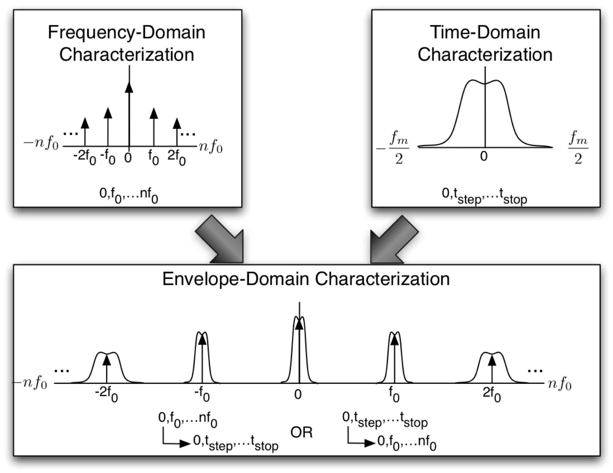 All measurements are captured as envelope signals Once the signal is captured, you can use various Fourier Transforms
to convert to other relatable signals.
Signal Transforms
| To \ From: | Envelope | Frequency | Time | Switching |
|---|---|---|---|---|
| Envelope |  = tf.tf( = tf.tf(  ) ) |
 = ff.tf( = ff.tf(  ) ) |
 = tt.tf( = tt.tf(  ) ) |
 = ft.tf( = ft.tf(  ) ) |
| Frequency |  = ff.ff( = ff.ff(  ) ) |
 = ff.ff( = ff.ff(  ) ) |
 = ff.ff( = ff.ff(  ) ) |
 = ff.ff( = ff.ff(  ) ) |
| Time |  = tt.tt( = tt.tt(  ) ) |
 = tt.tt( = tt.tt(  ) ) |
 = tt.tt( = tt.tt(  ) ) |
 = tt.tt( = tt.tt(  ) ) |
| Switching |  = ft.ft( = ft.ft(  ) ) |
 = ft.ft( = ft.ft(  ) ) |
 = ft.ft( = ft.ft(  ) ) |
 = ft.ft( = ft.ft(  ) ) |
The signals describe a nonlinear time-variant system as follows:
Envelope: Raw data capture.
Frequency: Frequency Spectrum waveform centered around each harmonic of a carrier frequency.
Time: Sub-Sampled waveform where each digital sample (\(\tau_t\)) contains analog sub-samples (\(\tau_f\)).
Switching: Analog switching behaviour computed over a slice of bandwidth (BW).
Units
To simplify data storage and manipulation, each mixed-signal is recorded in base-linear units:
Voltage: [\(V\)]
Current: [\(A\)]
Impedance: [\(\Omega\)]
Power [\(\sqrt{W}\)]
This ensures that all variables can be converted from base linear units to decibels (dB) using rW2dBW
Objects
An Object (such as an device) contains properties (such as signals). An object may also control the display, sweep limits, and optimization limits of each property using the following metadata:
obj.infoof typeAttributeInfo, which contains:
Infometadata for each object property.
obj.__info__(), a magic method that dynamically initializes theself.infometadata.
Devices
A Device AbstractDevice is an Object that contains:
DeviceClass.firmware_map, a static dictionary that contains supported device firmware information.
device.handles, a dictionary of device handles (any type) that uniquely describes a remote connection to the physical device(s).
device.connect_handles(), connects the device and stores device references inself.handles.
device.preset(), presets the device each time a unique connection is made.
device.disconnect_handles(), disconnects the device and removes device references fromself.handles.
device.infocontains display, sweep limit, and optimization limit meta-data.
Programming
Adding a Device Driver
Select the device(s) that best describe the instrument you want to control. Here are some common examples:
DC Supply
AWG
DAC
Multimeter
Oscilloscope
ADC
Open/Short Circuit
Varactor
Active Load
Signal Generator
VSG
AWG
Pulse Generator
SRD
VNA
VSA
Power-Meter
Oscilloscope
Sampling Scope
50 Ohms
Passive Load
Active Load
Select the device modulation complexity. For example, an RFSource can be inherit the following classes:
Write the driver.
Tip
It’s usually best to copy from previous drivers.
Tip
Store configuration data in a config file.
Tip
Complex instruments may require multiple drivers. Some high-end VNAs may contain:
LF Source
LF Receiver
RF Source
RF Receiver
Avoid repetition by programming common functionality in shared functions, such as:
preset()
arm()
trigger()
Register the driver by:
Place the source code file in the following search path:
sknrf/device/instrument/<device_type>/*
Place the config file in the following search path:
sknrf/data/config/device/instrument/<device_type>/*
Test the driver as follows:
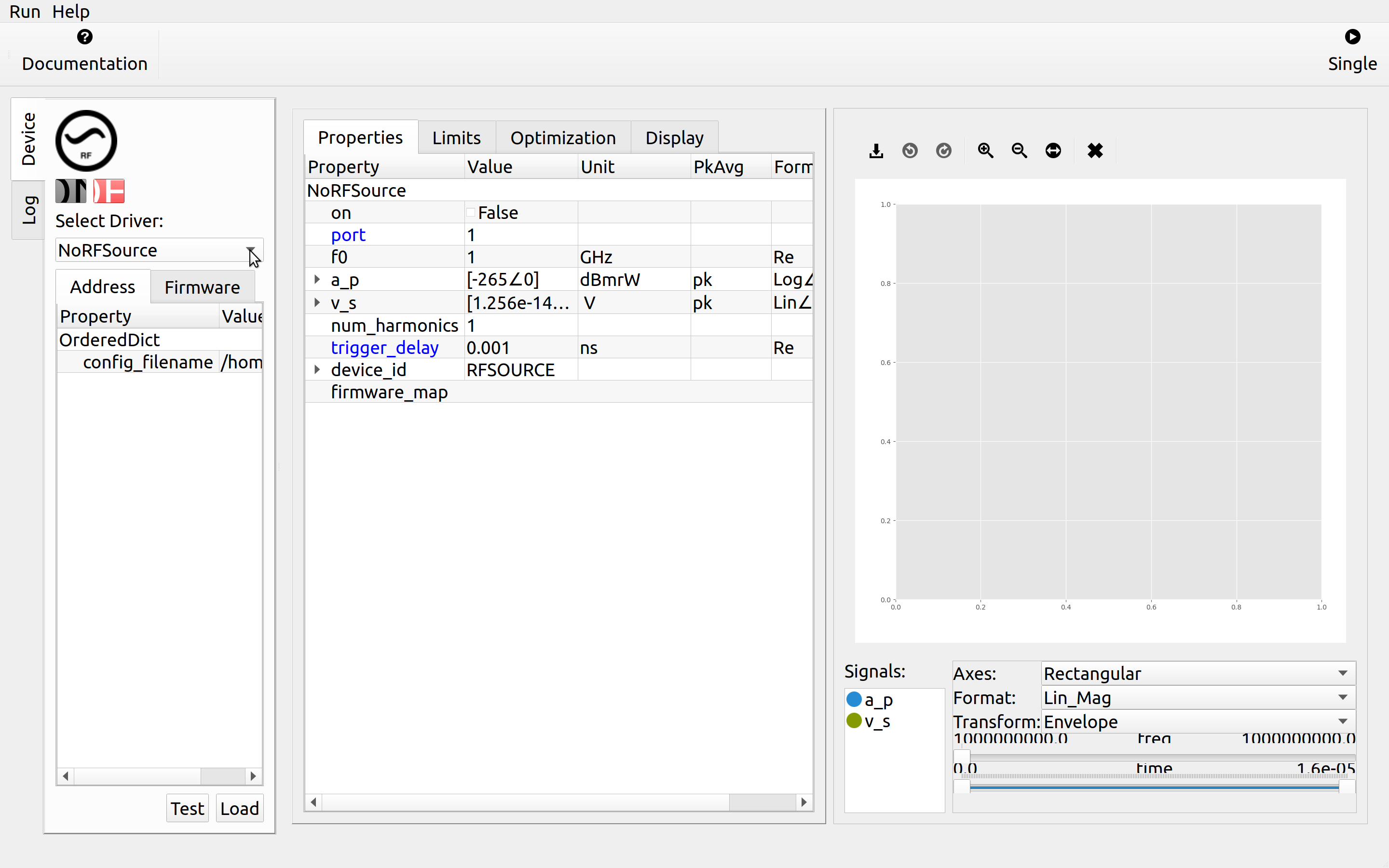
Select the driver
Modify the Address
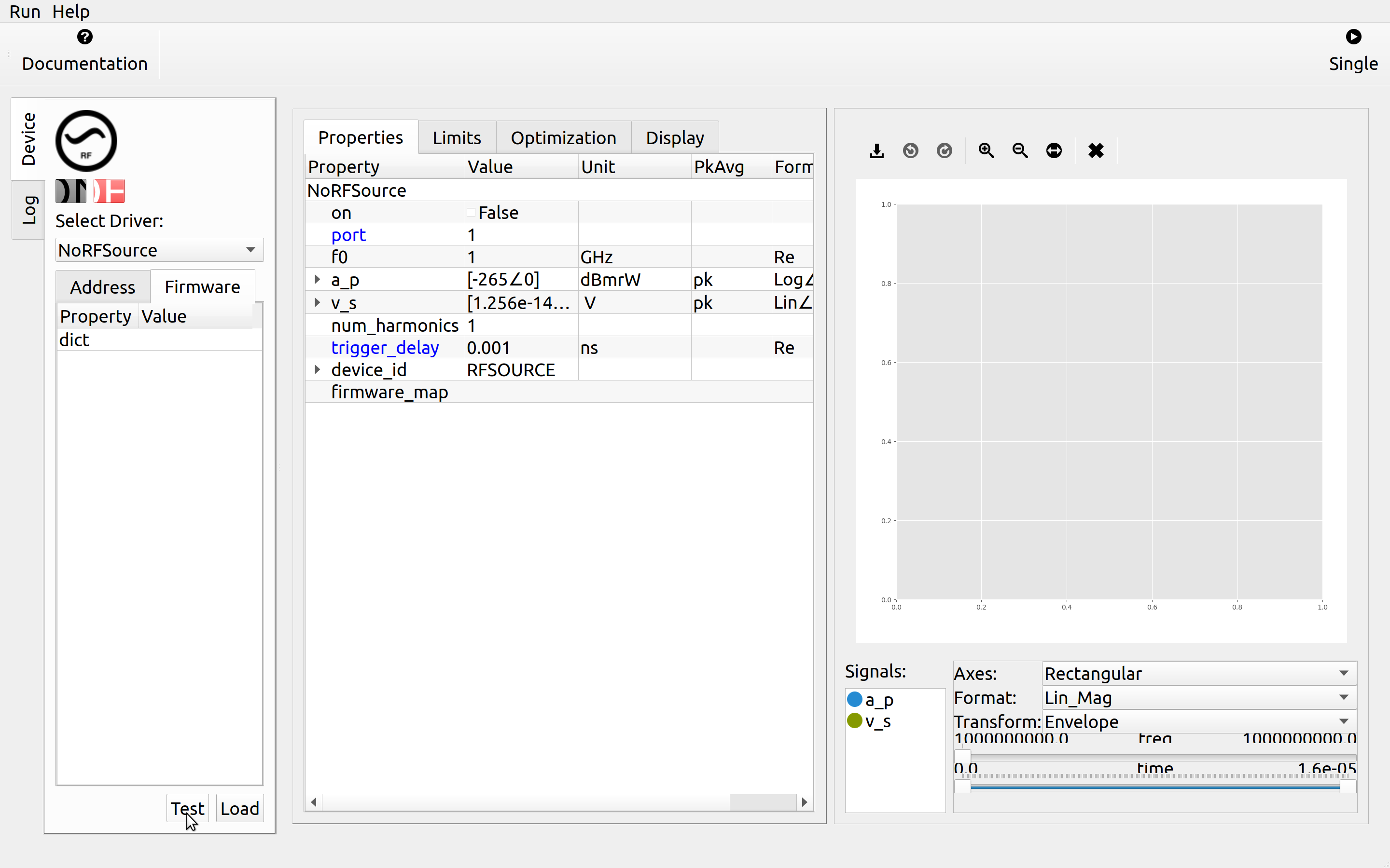
Verify the firmware versions match
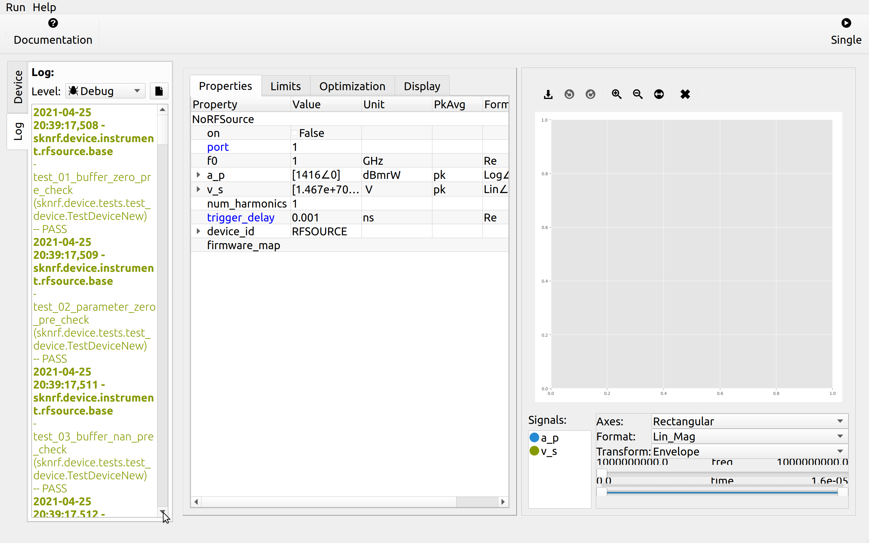
Test the driver
Load the driver
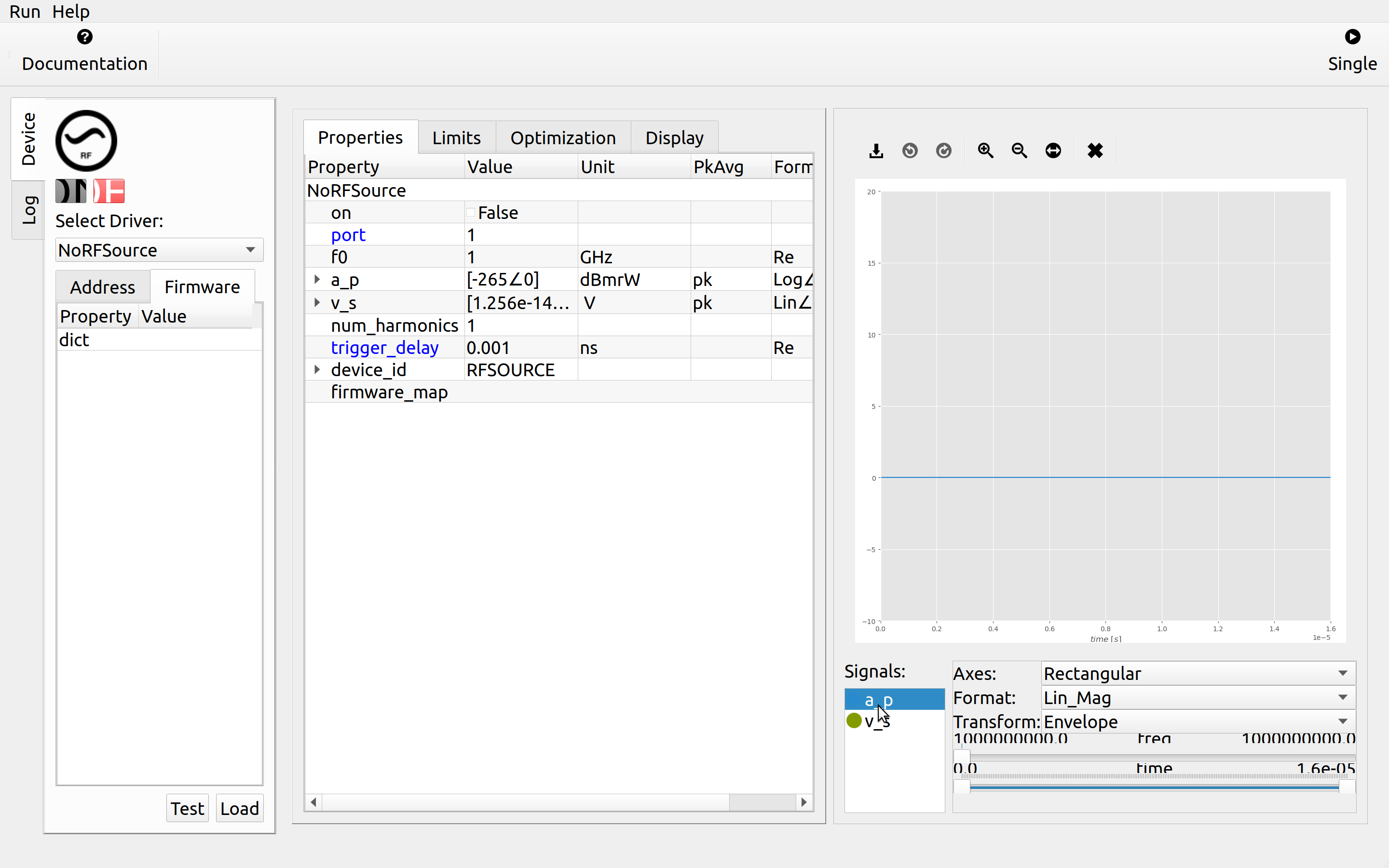
Run a Single Measurement
Plot the results.
API
The following is a minimal example of how to connect to an instrument:
from sknrf.device.base import AbstractDevice
from sknrf.device.instrument.lfsource.base import NoLFSource

AbstractModel.init()
dev = NoLFSource()


